In statistics, linear regression is a method of estimating the conditional expected value of one variable y given the values of some other variable or variables x. The variable of interest, y, is conventionally called the ‘response variable’. The terms ’endogenous variable’ and ‘output variable’ are also used. The other variables x are called the explanatory variables. The terms ’exogenous variables’ and ‘input variables’ are also used, along with ‘predictor variables’. The term independent variables is sometimes used, but should be avoided as the variables are not neccessarily statistically independent. The explanatory and response variables may be scalars or vectors. Multiple regression includes cases with more than one explanatory variable.
The earliest form of linear regression was the method of least squares, which was published by Legendre in 1805, and by Gauss in 1809. Legendre and Gauss both applied the method to the problem of determining, from astronomical observations, the orbits of bodies about the sun. Euler had worked on the same problem (1748) without success. Gauss published a further development of the theory of least squares in 1821, including a version of the Gauss-Markov theorem.
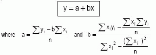
A regression of y on x is a way of predicting values of y when values of x are given. If the regression is based on a straight line graph, it is called a linear regression, and the straight line is called the regression line. The regression line (sometimes referred to as the line of best fit) of y on x is then the line that gives the best prediction of values of y from those of x, and is:

n being the number of data pairs. (Note that the regression line of x on y, which is usually different from the regression line of y on x, can be found by interchanging x and y in the above expressions). a and b are known as the linear regression coefficients. The independent variable is the regressor, and the dependent variables is called regressand. The coefficients are found by minimizing the sum of the squares of the vertical distances of the points from the line (i.e. the sum of the squares of the residuals). This method is known as least squares.
The correlation coefficient is a measure of the amount of agreement between the x and y variables, and is given by:

When r is positive, the correlation is positive, which means that high values of one variable correspond to high values of the other. Conversely, if r is negative then the correlation is negative: low values of one variable correspond to high values of the other. An important property of r is that -1 d r d 1. The ±1 values correspond to a perfect correlation: real values and estimates are exactly the same. If r = 0 then there’s no correlation: x and y are uncorrelated.
 Non-Linear Regression Models
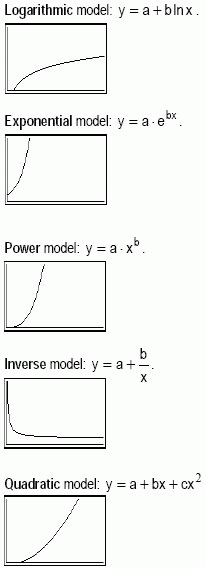
In addition to the linear regression more types of regression of a variable y on a variable x, namely:
Logarithmic model: The logarithmic curve-fitting model requires positive x-values. An example of this model is the psychophysics law of Weber-Fechner.
Exponential model: This model requires positive y-values. Examples of this model are the number of undecayed nuclei of radioactive materials after a period x of time, the discharging process in Capacitor-Resistance circuits, etc.
Power model: The power model requires positive x-values and positive y-values, otherwise the DOMAIN error occurs when attempting to display the STATVAR menu. Newton’s law of gravitation is a classic example.
Inverse model: Zero cannot be one of the x-values, since it will trigger the DIVIDE BY 0. Examples are Curie-Weiss’ law, the reactance of a capacitor, relation between potential energy and distance, etc.
Quadratic model: Bear in mind that this model needs at least three points. An example is the relation between kinetic energy and speed.
Reference: en.wikipedia.org/wiki/Linear_regression